Aws
March 2023
Data science in the cloud (AWS)
Overview
In this practical we will introduce the cloud compute environment used during the course. While it is possible to work on your own machine, some practicals will use GPU-accelerated deep learning. Cloud-based systems allow us to easily provision the required resources and break them down again once we’re finished. You can also access the cloud environment from anywhere, without needing a powerful machine yourself.
AWS Sagemaker
We will use the AWS Sagemaker Studio environment. It is web-based and accessed through the browser, similar to Jupyter Lab/Notebook. Follow the steps below to get started.
Getting started
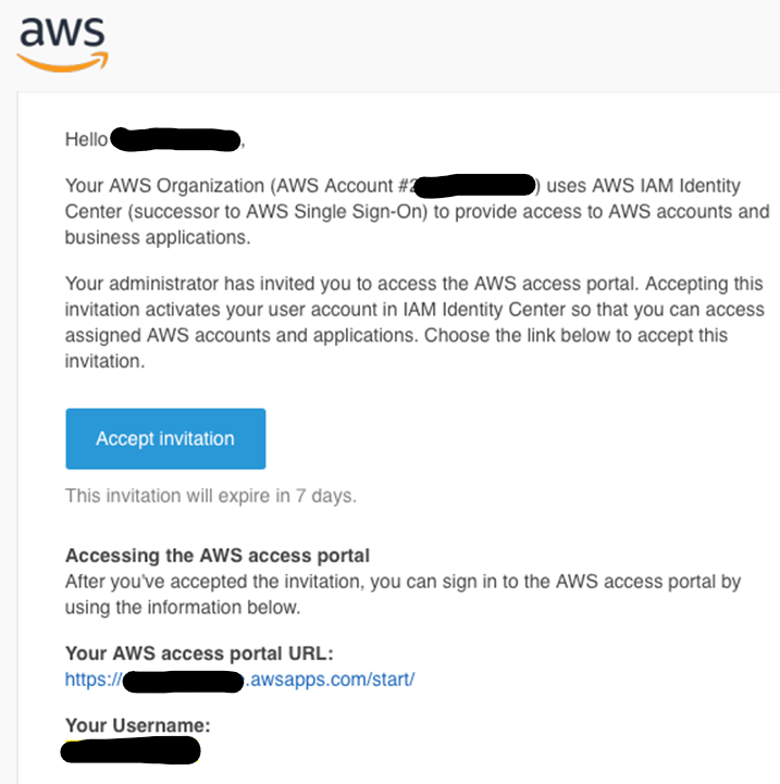
You will have received an email with an invitation link to the AWS environment. Accept the invitation and create your password. You can then use the AWS access portal URL from the email to access the Studio environment, look for the link in the format https://xxx.awsapps.com/start/
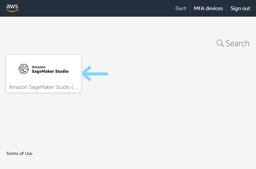
Log in with your assigned username and your chosen password. You will see a screen like this - click on the Sagemaker Studio button to start.
Sagemaker Studio
After logging in you will be presented with a home screen. Click on the folder icon on the left to access your workspace.
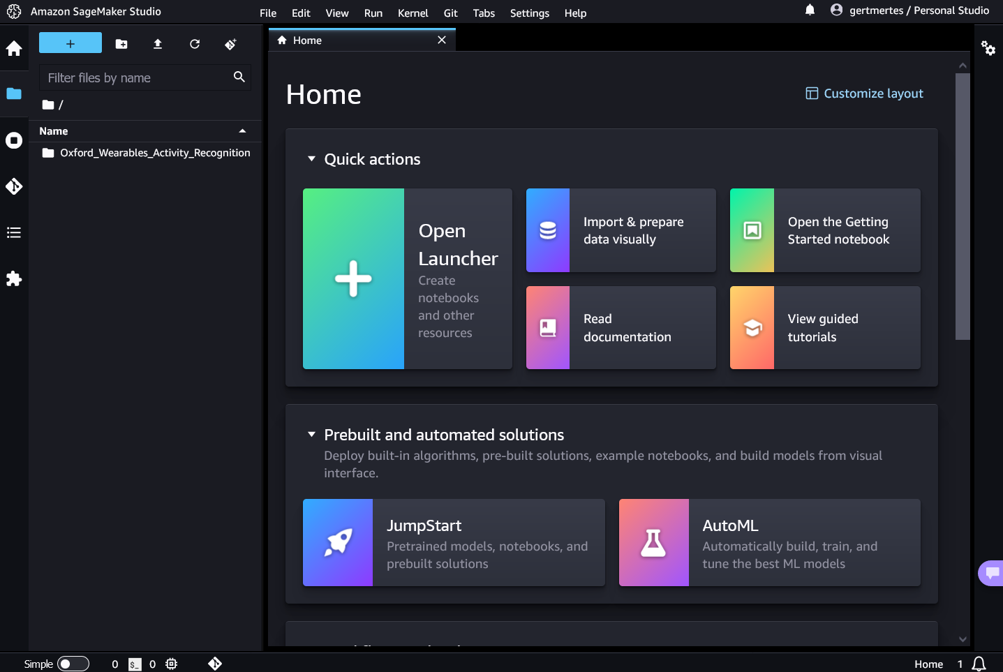
On the left side you see your workspace. There should already be a folder there containing the course material. But for now, stay in your root directory /.
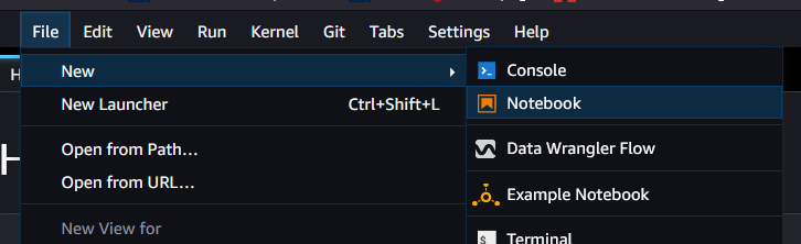
Go to File -> New -> Notebook to create a new Jupyter notebook. This will create a new notebook Untitled.ipynb (you can change the name later).
When opening a notebook for the first time, the following popup will show:
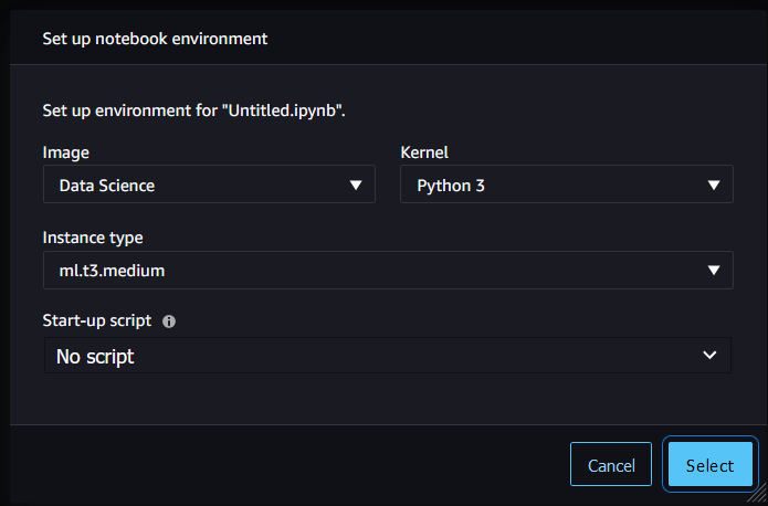
Here you define the compute environment the notebook will run in.
- Image: The image defines a set of pre-installed software on the underlying system. For most practicals in the workshop, use the Data Science image. For the Deep Learning and PyTorch practical, use the PyTorch 1.12 Python 3.8 GPU image.
- Instance type: This sets the compute resources available (CPU, RAM and GPU). Your tutor will instruct you which one to select during the workshop. For now, select ml.t3.medium (2 CPUs + 4GB)
- Leave Start-up script as default. This will automatically install the required python dependencies.
After pressing select, the environment (kernel) will start - this can take a minute.
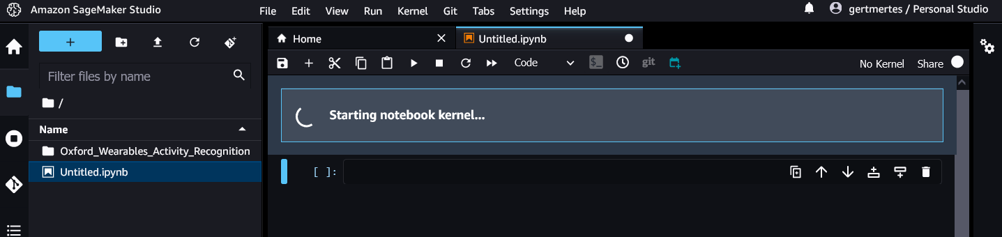
When it’s done, you will have a working Jupyter notebook running on a virtual machine with 2CPUs, 4GB RAM, preinstalled with common Data Science packages (numpy, pandas, etc) and the ones used during the workshop.
It’s important to understand the distinction between the notebook and the compute environment. The notebook is the front end, the compute environment is the backend - that is, the system the code is running on. The python server in charge of running the code is called a kernel.
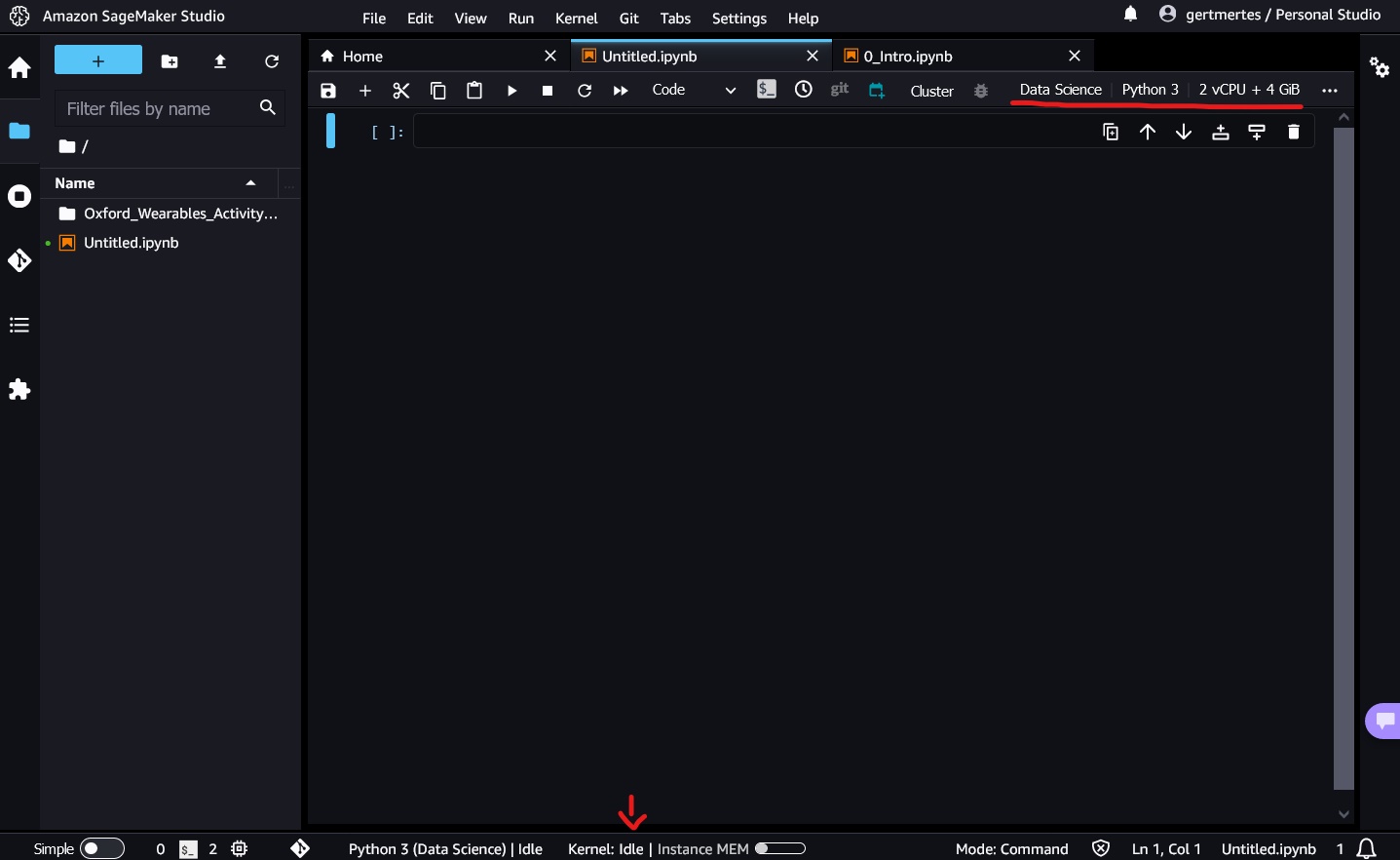
The notebook we just created is now running on the machine type we selected. You can run multiple notebooks on the same compute instance - simply select the same Image and Instance type when starting the notebook. In the top right corner of the notebook, you will see information about the current running kernel and system.
Running instances
Closing your notebook does not stop the machine and kernel it is running on. You can open the notebook again and continue where you left off. Click on the circular icon on the left to open the Running Instances tab.
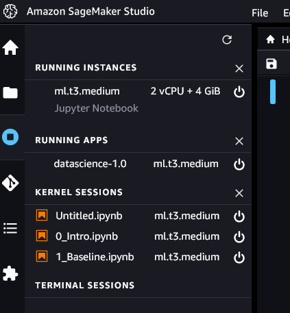
This tells you which instances and kernels are currently active.
- Running Instances: currently running virtual machines
- Running Apps: currently active software environments
- Kernel Sessions: currently active kernels. This corresponds to a “running notebook”. You can double click on the notebook to open it and you will continue where you left off.
In the above example, all of the active notebooks are running on the same virtual machine (ml.t3.medium).
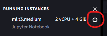
Shutdown instances
At the end of each practical you should shut down all running instances. Click on the power icon next to the running instance. This will shut down the running instance as well as any notebooks running on it. Make sure so save your notebooks before shutting down the instance. Next time you open a notebook, you simply start the instance again.
Jupyter Notebook
Your code will live in a Jupyter Notebook, also simply called a notebook. Notebooks are self-contained interactive python environments that contain code and output, and can also contain text (markdown). The output in a notebook is persistent. Once code is executed and the output shown/rendered, it is saved in the notebook. The notebook can then be closed and shared with others, without needing to be executed again.
Cells
Notebook code lives in cells. These are small snippets of code used to structure your work. Cells typically contain code that does a single task and print or plot some output. They’re useful for calculating and printing intermediary results or debugging output. Below is a simple example, copy the code into the first cell.
import numpy as np
import matplotlib.pyplot as plt
%matplotlib inline

x = np.random.randn(20)
plt.plot(x)
Execute the cell with Shift+Enter (or by pressing the play button). This will run the cell and automatically create a new one below it.
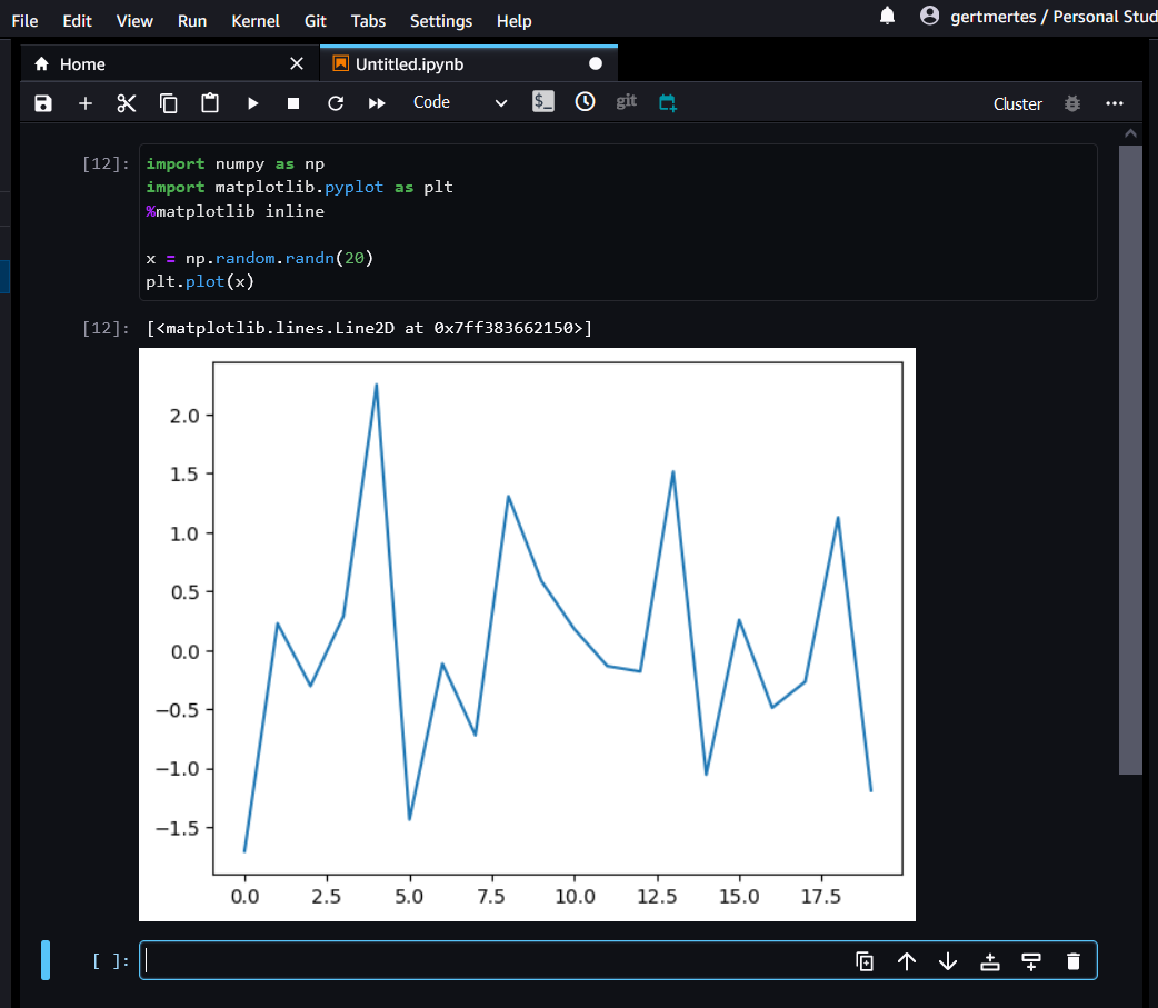
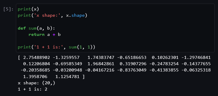
As you can see, the cell’s output (in this case a plot) is shown below it. Use cells to structure your code and display intermediary output. To investigate variables, you can simply use the print() function, as shown in the example below. You can also declare and use functions just like in regular python scripts.
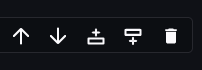
You can create new cells using the + button. This will create a cell below the currently selected one.
The buttons on the right side of the cell can also be used to move the cell up or down, or create new cells above or below the selected one. Delete the cell with the trashcan icon.
For long running cells, you can see the status at the bottom. When it says “Kernel: Busy” it means your code is still executing.
Cells can be split or merged using the Right Click menu (right click inside the cell body). To split a cell, put the cursor on the line you want to split at, then Right Click -> Split Cell. Similarly, to merge a cell select Right Click -> Merge call above/below to merge with the cell above or below.
Useful Shortcuts and Commands
Ctrl + EnterRun the current cell.Shift + EnterRun the current cell and advance to the next one. If you are in a last cell, a new cell will be inserted at the end.Alt + EnterRun the current cell and insert a new one below.TabCode completion. Start typing the name of a function, and pressTabto autocomplete it. If there is more than 1 option, it will show all available. Note: this requires the notebook to be running and the module/functions need to be imported first.Shift + TabShow a documentation popup of the module or function at the cursor’s current location. Useful to see function arguments (click on a function and press the shortcut).Ctrl + ZUndo-
Ctrl + Shift + ZRedo - Run -> Run All Cells
- Run -> Run Selected Cell and All Below
- Kernel -> Interrupt Kernel: to stop executing code (e.g.: to stop a for loop)
- Kernel -> Restart Kernel: Useful if your code hangs and Interrupt doesn’t work. This clears everything in memory, so you will need to run the notebook from the beginning again.
- Edit for cell operations (or right-click on a cell)