Prac3 Data Analytics
November 2021
- Tools needed
- 1. Setup and installation
- 2. Extracting data
- 3: Preprocessing
- 4. Visualising your data (optional)
- 5. Returning your camera and accelerometer
In this practical, you will process data collected from your accelerometer.
Tools needed
- Conda /Virtualenv to manage depedencies
- Java 8+: Download jdk-17 here. If you are on a Mac machine, make sure to select the right distribution for the chip you have. For m1 chips, get arm64. For intel chips, get x64.
1. Setup and installation
First we need to install a package that can pre-process your accelerometer data. To do this, activate your virtual environment either using conda or virtualenv.
Conda activation
$ conda create -n acc_parsing
$ conda activate acc_parsing
or virtualenv activation
$ pip install virtualenv
$ virtualenv acc_parsing
$ source acc_parsing/bin/activate
Once your envrionment has been activated, install the package using pip:
$ pip install accelerometer
You should keep your environment active for the remaining for the practical.
2. Extracting data
We will now extract the raw data from your accelerometer device.
Accelerometer
- Plug in your accelerometer to your computer. Go to the external drive where it is located and copy the .CWA drive
over wherever you want. Rename the file as
myAcc.cwa.
$ cp /Volumes/AX317_41145/CWA-DATA.CWA ~/practicals/data/myAcc.cwa
-
Safely disconnect the device and put your accelerometer back on!
-
Currently the raw data stored in the CWA file does not allow easy extraction of the 3-axis acceleration data, so we need to convert this to a more suitable format such as CSV for furthur manipulation. Run the following in your
practicalsfolder:$ cd ~/practicals $ accProcess data/myAcc.cwa --rawOutput True --activityClassification False --deleteIntermediateFiles False
3: Preprocessing
In this practical, we will focus on the preprocessing steps performed on your accelerometer data for activity recognition. This is an often time-consuming, yet very important, step before your data is useful for further analysis. You are provided with a half-completed jupyter notebook to work with.
After this you will use our built pipeline and perform activity recognition on your accelerometer data with machine learning.
Buillding features from your accelerometer traces
Your raw accelerometer traces are now in practicals/data/myAcc.csv.gz. It contains 4 columns: time, x, y and z accelerometer readings.
Go through the jupyter notebook Features.ipynb in practicals/scripts.
Biobank Pipeline
While you have had a taste of raw sensor data preprocessing through the jupyter notebook, many other operations (such as readings imputation, non-wear time detection ..) can be done on your raw data to further improve your dataset for downstream machine learning tasks.
So instead of using the dataset you just created, my_data.csv, we will now go back to your raw data again - the CWA file. We will run some scripts which form the standard analysis pipeline on accelerometer data in the Biobank studies such as this paper. This involves preprocessing operations as well as running a machine learning model that had been trained on the Biobank data for activity recognition.
Note that these operations also involve mapping the fine-grained annotations you had into larger classes. You shall still be in the practical folder.
$ accProcess data/myAcc.cwa --useFilter False
To visualise the time series and activity classification output:
$ accPlot data/myAcc-timeSeries.csv.gz data/plot.png
Now unzip your .csv.gz file if you haven’t done so already.
gunzip data/myAcc-timeSeries.csv.gz
Finally, we want to check the model predictions against your true annotations.
$ python3 scripts/check_annotations.py /data/myAcc-timeSeries.csv data/me-annotation.csv --plotFile check_results.png
Inspect plot.png in your data folder and various .png generated in your prac3 folder to see how the model has done!
4. Visualising your data (optional)
For this practical, we wish for you to produce some visualisations to share in a presentation. This practical is open-ended in nature, you can explore any topic as the basis of your visualisation according to your interests.
Timeline
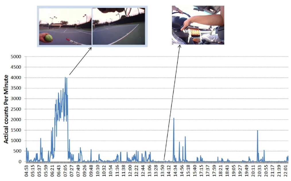
Prepare a timeline to illustrate your days.
Taken from Nature news feature ‘The lab that knows where your time really goes’

From ‘Using wearable cameras to categorise type and context of accelerometer-identified episodes of physical activity’, Doherty et al.

From ‘Wearable camera-derived microenvironments in relation to personal exposure to PM2.5’, Salmon et al.

Side-by-side
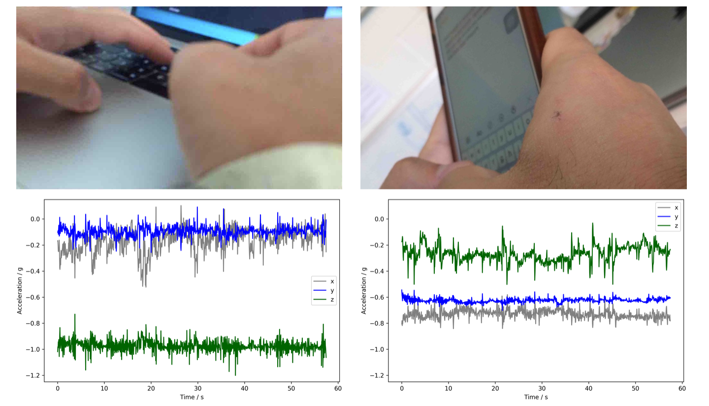
Compare the data captured by the two devices (camera vs accelerometer) when you are performing different activities. Prepare a table of different activities, e.g. ‘sitting’, ‘eating’, ‘walking’ and show a side-by-side comparison of the two sources of data.
Here is a comparison of the activities ‘typing on computer Vs. typing on phone’ as captured by the two devices. ‘Are Accelerometers for Activity Recognition a Dead-end?’, Tong et al.


Propose your own task
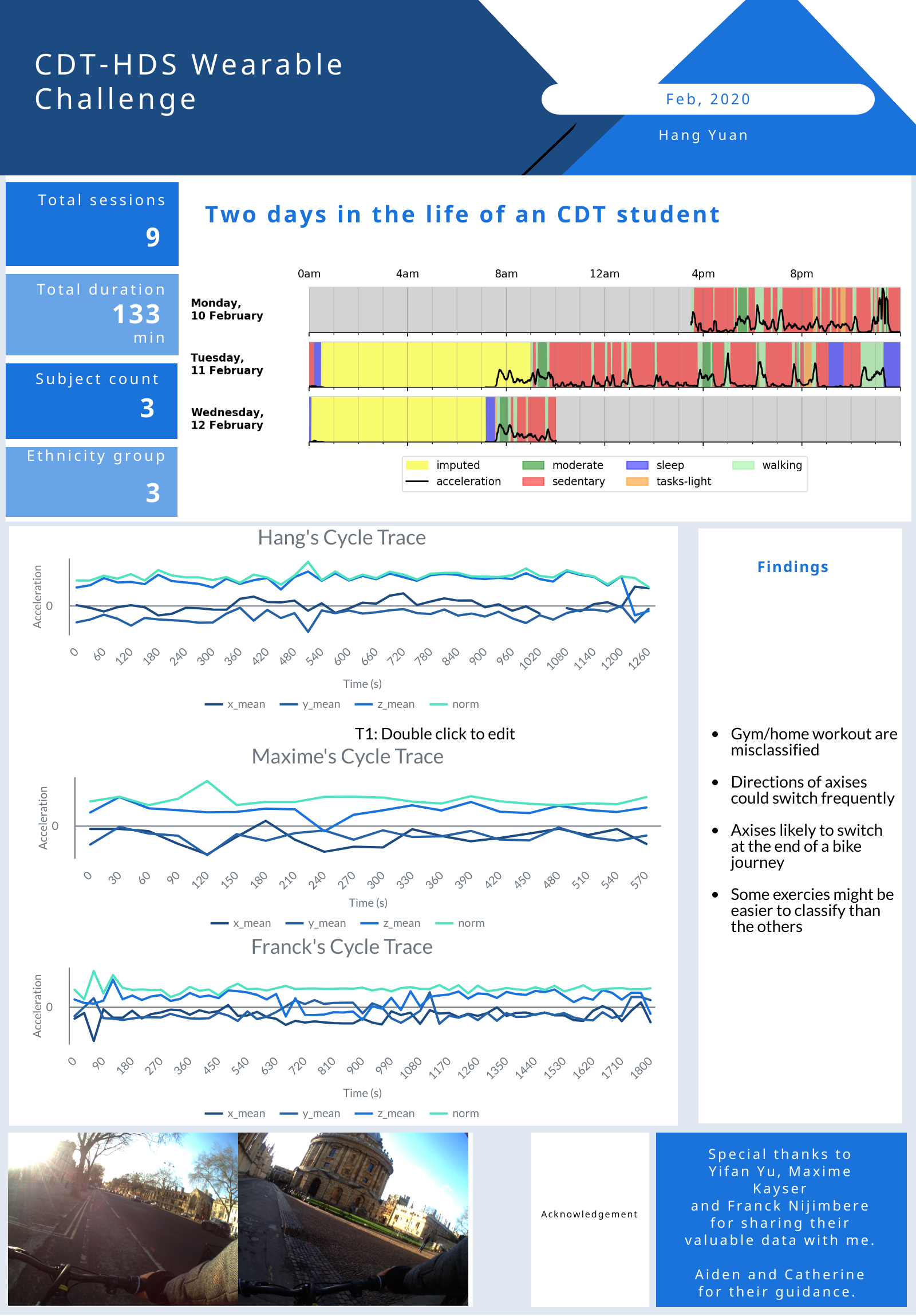
The above is an example from last year.
If none of the above visualisations inspire you, feel free to propose and pursue your own idea.
Some ideas might be:
-
Compare the different annotation schema you had used
-
Look into the distribution of activities in your data
5. Returning your camera and accelerometer
You should have loaded your images onto your computer by now so you can safely delete the data from you camera!
Plug your camera in, and navigate to the utilities folder within oxford-wearable-camera-browser and type the following:
$ cd ~/oxford-wearable-camera-browser/utilities/
$ python3 autographer.py --delete True
Plug your accelerometer in, and delete the .CWA file:
$ rm /Volumes/AX317_41145/CWA-DATA.CWA
Handin: Return the camera and accelerometer to your tutor before you leave.