Tutorial 03
Probe health with day-level embeddings
Aggregate valid Sensori days into participant representations and test what they add beyond age, sex and BMI.
Minute embeddings describe short behaviours. For health inference, Sensori
instead encodes each valid 24-hour recording and combines repeated days into
one participant representation. This tutorial pairs the day arrays from
tutorials/nhanes_preprocessing.ipynb with public NHANES questionnaire and
examination data.
Prepare the analysis data
This tutorial needs two inputs, prepared separately.
The day arrays come from tutorials/nhanes_preprocessing.ipynb, which downloads
public NHANES participants and writes day_*.npy for each of them. Point
day_data_dir at the directory it produced.
The tabular variables come from prepare_tabular(), which downloads the public
NHANES questionnaire and examination tables for both survey cycles and keeps the
participants who have public accelerometer data:
from pathlib import Path

from scripts.tutorial_nhanes.prepare_nhanes_tabular import prepare_tabular

work_dir = Path("/path/to/nhanes-workspace")
day_data_dir = Path("/path/to/processed-nhanes-days")

tabular = prepare_tabular()
The resulting table includes age, sex, BMI, health variables, physical-function items, survey cycle and monitor firmware.
Extract day embeddings
The standard inference loader receives every 24-hour NPY file as input, regroups
it into 1-minute model windows and returns one 768-dimensional embedding per
valid day. On first use, the pretrained model weights and model config file are
downloaded to checkpoint/ in the cloned Sensori repository.
import torch

from sensori.inference import extract_embeddings

embedding_path = work_dir / "nhanes_embeddings.npy"
extract_embeddings(
    day_data_dir,
    output_path=embedding_path,
    accelerator="gpu" if torch.cuda.is_available() else "cpu",
    batch_size=100,
    num_workers=6,
)
The saved NumPy object groups day embeddings by participant; existing output is reused.
Aggregate participants
Normalize each finite, non-zero day embedding to unit length before averaging
across a participant’s available days. This gives each day equal directional
weight and produces one [768] vector per participant.
import numpy as np

day_embeddings = np.load(embedding_path, allow_pickle=True).item()
participant_embeddings = {}

for participant, values in day_embeddings.items():
    values = np.asarray(values, dtype=np.float32)
    norms = np.linalg.norm(values, axis=1)
    valid = np.isfinite(values).all(axis=1) & (norms > 0)
    if valid.any():
        participant_embeddings[str(participant)] = (
            values[valid] / norms[valid, None]
        ).mean(axis=0)
The notebook goes further: it turns this dictionary into a table and inner-joins it with the NHANES variables, so the analysis cohort is the participants who have both tabular data and at least one valid day embedding.
Fit health probes
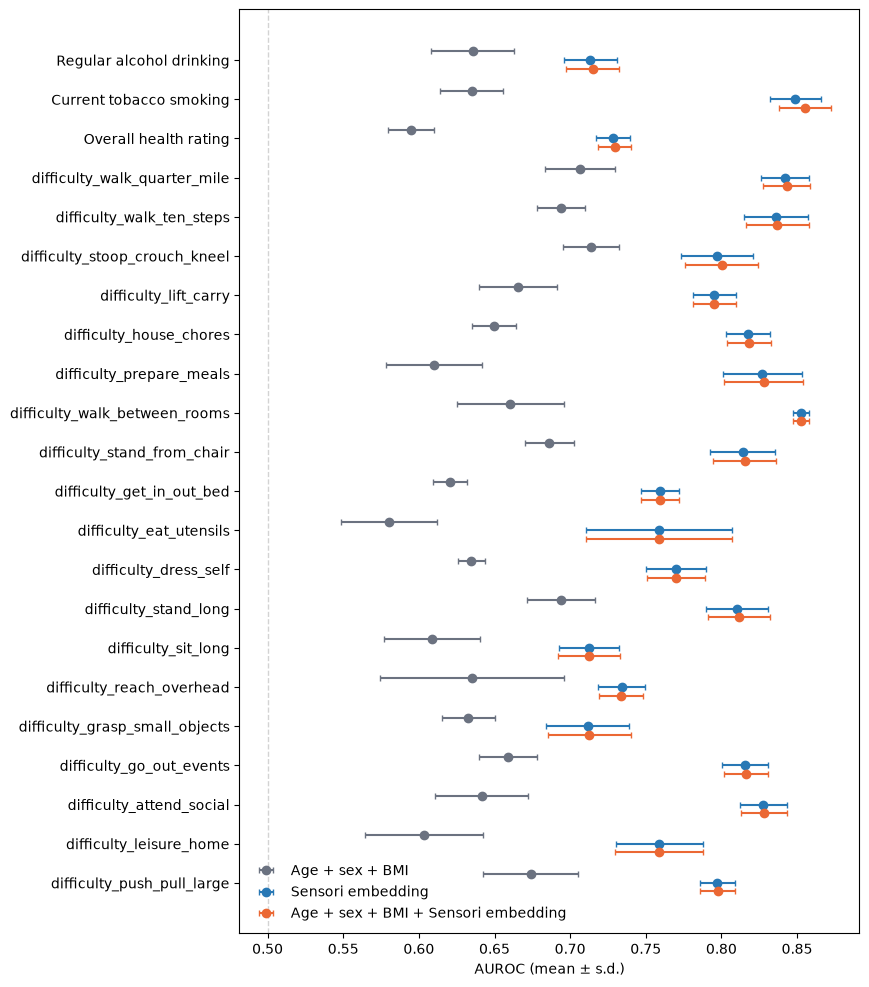
To reproduce the notebook benchmark, retain participants aged 43–79 years and encode three harmonized health outcomes—regular alcohol drinking, current tobacco smoking and overall health rating—plus 19 physical-function outcomes.
Three logistic-regression probes are compared on the same target-specific participants and five stratified folds:
- age, sex and BMI
- Sensori embedding
- age, sex, BMI and Sensori embedding
Imputation and standardization are fitted inside each training fold. The notebook reports AUROC; its summary shows the mean and standard deviation across folds.
Interpret the results
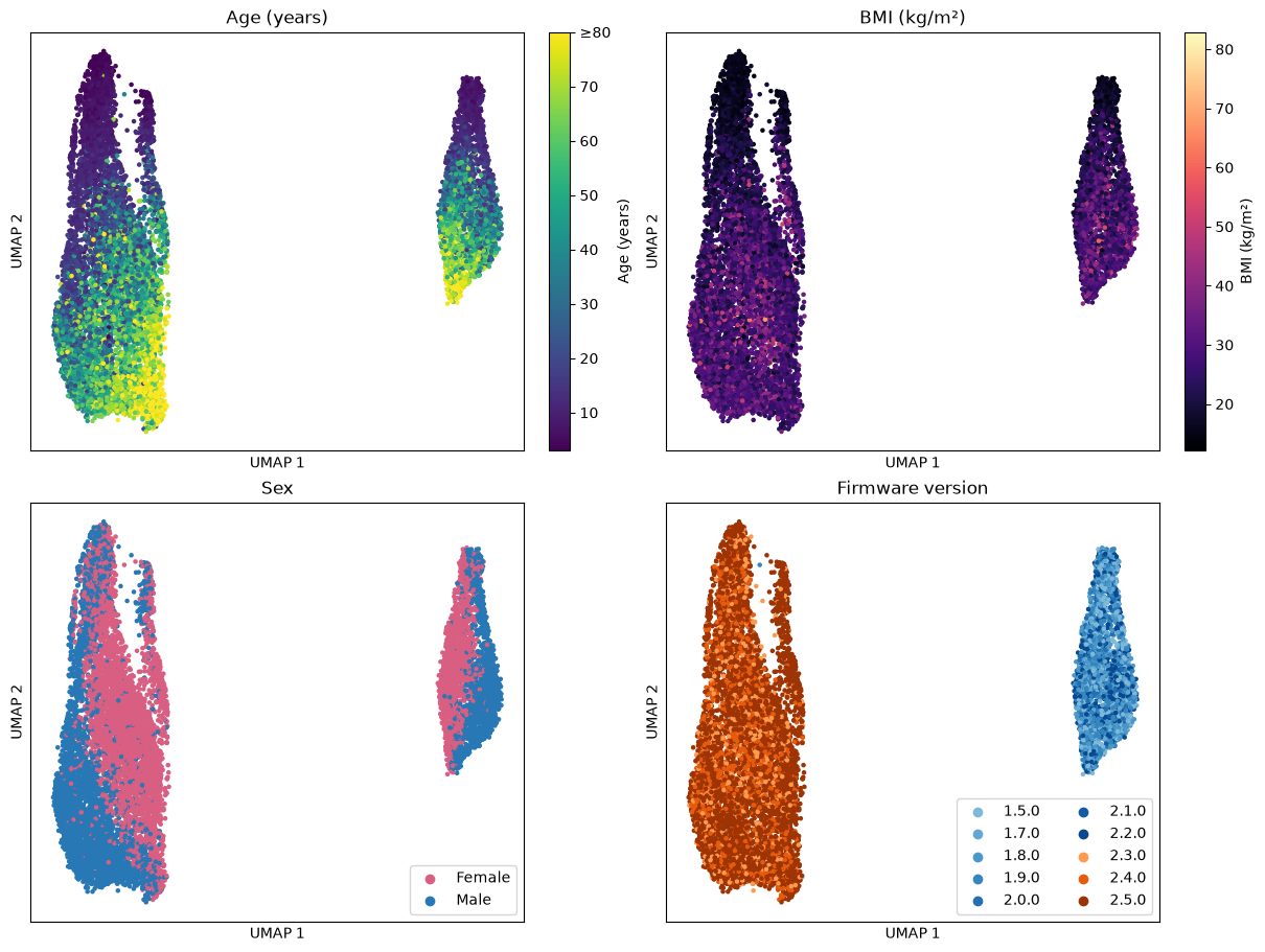
The embedding-only UMAP is annotated with variables that Sensori never saw. Age, sex and BMI vary within the representation; the strongest split is monitor firmware. Changes to the device’s idle sleep mode alter the waveform during sleep and non-wear, creating a visible data distribution signature.
The outcome plot compares the three feature sets. Blue and coral points show what the Sensori representation captures alone and beyond demographics; horizontal bars are the sample standard deviation across five folds, not confidence intervals.