Recognise activities minute by minute

This tutorial moves from complete days to short, labelled behaviours. It uses public HAR datasets with their own preprocessing pipeline, so you do not need the daily NPY files created in Tutorial 01. You need an installed Sensori repository, network access for the initial downloads and enough disk space for the source datasets.

Depending on the temporal scale of interest, one can totally extract embedding at other temporal dimensions for downstream evaluation.

Prepare public datasets

The notebook tutorials/har_evaluation.ipynb prepares PAMAP2, RealWorld and WISDM by default. Missing datasets are downloaded from their official release. Each recording is split into 60-second windows with a 30-second overlap, producing an acceleration array (X.npy), an activity label for every window (Y.npy) and its participant key (pid.npy). Capture24 uses the same interface and can be added when required.

from pathlib import Path

from scripts.tutorial_har.prepare_all_datasets import prepare_datasets

work_dir = Path("/path/to/har-workspace")
datasets = ("PAMAP2", "RealWorld", "WISDM")

dataset_paths = prepare_datasets(
    work_dir,
    datasets=datasets,
    epoch_len=60,
    overlap=30,
)

Extract minute embeddings

Sensori low-pass filters each window at 5 Hz, resamples it to 10 Hz and passes the resulting [600, 3] signal through the frozen convolutional encoder. The output is one 512-dimensional embedding per 60-second window. On first use, the pretrained model weights and model config file will be downloaded to checkpoint/ in the cloned Sensori repository.

from scripts.tutorial_har.extract_har_features import extract_embeddings

embedding_paths = extract_embeddings(
    "sensori",
    dataset_paths,
    work_dir / "embeddings",
    batch_size=256,
)

A GPU is used when available; otherwise extraction runs on the CPU. Each saved array has shape [windows, 512], with rows aligned to the corresponding labels and participant keys.

Evaluate without leakage

The same participant can contribute many overlapping windows. A random window-level split would therefore put nearly identical observations on both sides of the evaluation. The notebook instead keeps every participant wholly inside one fold.

The regularization strength is chosen by nested cross-validation: an inner participant-grouped grid search scored by macro-F1, then evaluation on participants the search never saw. The summary reports macro-F1 and Cohen’s κ as the mean and standard deviation across outer folds.

Dataset	Macro-F1, mean ± s.d.	Cohen’s κ, mean ± s.d.	Selected `C` by fold
PAMAP2	0.848 ± 0.071	0.842 ± 0.071	10; 100; 100; 0.1; 0.1
RealWorld	0.863 ± 0.023	0.826 ± 0.031	0.1; 0.1; 0.1; 0.1; 1
WISDM	0.815 ± 0.080	0.805 ± 0.083	0.1 in all folds

Mean macro-F1 ranges from 0.815 on WISDM to 0.863 on RealWorld, while mean Cohen’s κ ranges from 0.805 to 0.842 across the three datasets.

All rows use frozen Sensori embeddings and five outer folds. C was selected independently inside each outer fold, so its values can vary across folds.

This design tests whether activity labels are linearly accessible from frozen minute embeddings. It does not fine-tune Sensori, and activity labels are not harmonized across datasets.

Inspect the embedding space

The notebook also fits UMAP to the Sensori embeddings. Nearby points represent windows with similar learned features; colour is added afterward from the activity labels.

UMAP of PAMAP2 minute embeddings, coloured by eight activities including walking, sitting and stair use. — PAMAP2. Walking, postural activities and stair use occupy distinct but connected regions.

UMAP of RealWorld minute embeddings, coloured by activities including walking, running, sitting and climbing stairs. — RealWorld. The map separates locomotion and postural behaviours while retaining within-class variation.

UMAP of WISDM minute embeddings, coloured by eighteen everyday and sporting activities. — WISDM. A broader activity vocabulary produces several compact clusters and overlapping everyday behaviours.

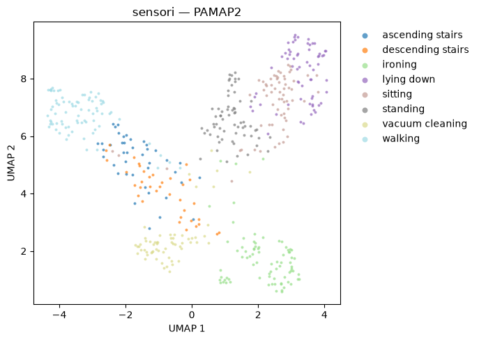
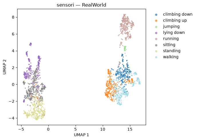
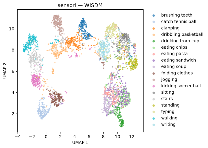
UMAP is a descriptive view, not a performance estimate: distances and cluster shapes depend on its settings. Use the participant-grouped linear-probe metrics—not visual separation—to compare representations.